Monochromator alignment and calibration

Energy calibration background

The X-ray beam produced by the elliptically polarized undulator (EPU) is a white beam that consists of a broad distribution of energies. The beamline uses a plane grating monochromator (PGM) to diffract the white beam into its constituent energies. The angle of the PGM along with the location and size of an exit slit aperture determines which beam energy goes down the beamline.

Anytime the PGM is translated in the X (inboard-outboard) direction, its rotation angle needs to be calibrated because the X motor does not precisely return to the same location on the PGM, and the beam energy is very sensitive to even slight offsets in the PGM angle. The PGM angle is calibrated on the basis of the grating equation:

\[m\lambda = d(\sin\alpha + \sin\beta)\]

In this equation, \(m\) is an integer that represents the diffraction order, \(\lambda\) is the wavelength of the incident light, \(d\) is the grating spacing (the distance between adjacent grooves), \(\alpha\) is the angle of incidence of the light (from the grating normal), and \(\beta\) is the angle of the diffracted light. If \(\alpha\) and \(\beta\) are on opposite sides of the grating normal, they will have opposite signs. To learn how the grating equation is derived, expand the section below.

TODO: The actual grating used by RSoXS is a variable-line-space (VLS) grating, so \(d\) is no longer constant. However, Eliot’s codebase still uses the above simplified form of the grating equation. Get clarification. Are the other gratings used variable-line spacing? If so, are these equations correct there and just being translated to RSoXS grating as well? Eliot might have mentioned that we only use the 250 l/mm portion of the RSoXS grating, but I also have read elsewhere that the VLS is meant to use all spacings together.

Deriving the grating equation

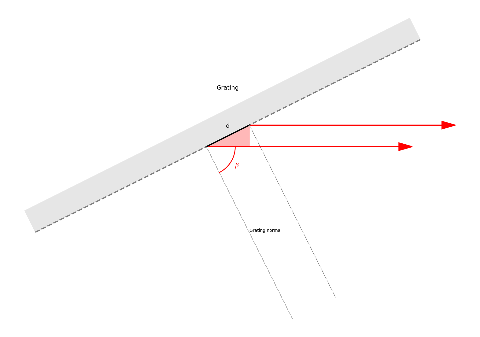
The derivation of the grating equation is very similar to the derivation of Bragg’s law. Imagine a ray of light hitting one groove on the grating, and a parallel ray of light hitting the adjacent groove that is length \(d\) away. Both rays have an incident angle of \(\alpha\) and diffracted angle of \(\beta\).

This drawing shows a sketch of the inboard side of the beamline. The diffracted beam always points to the right because it represents the portion of the diffracted beam that goes down the beamline and is measured by downstream detectors. In reality, there will be diffracted (and reflected, 0-order) rays of light going at a variety of angles because the incident beam is a white beam, and the diffracted rays represent a monochromatic beam. However, only the diffracted rays that go down the beamline can be meaningfully measured and calibrated.

It is also noted that the PGM diffracts light in a grazing incidence geometry rather than in a transmission geometry. This is because grazing at shallow angles maximizes the beam flux that goes down the beamline, whereas larger angles of incidence would result in a larger fraction of the beam flux being absorbed by the PGM and other optics.

```{python}
#| code-fold: true
import numpy as np
import matplotlib.pyplot as plt
import matplotlib.patches as patches

"""
## TODO: write code in own words, and remove the unnecessary parameters

## Define grating geometry
d_grating_spacing = 1.0
slope_grating = 0.5
y_intercept_grating = 2.0
length_grating = 8.0
height_grating = 0.5

## Define line along the bottom of the grating
x_coordinates_along_grating = np.array([-length_grating/2, length_grating/2]) ## Center of grating is 0, endpoints are ends of the bottom of the grating
y_coordinates_along_grating_bottom = slope_grating * x_coordinates_along_grating + y_intercept_grating
"""


## Generated from AI

# ---------- Parameters ----------
d = 1.0
grazing_angle_deg = 15.0
grazing_angle_rad = np.deg2rad(grazing_angle_deg)

m = 0.5
b = 2.0
grating_length = 8.0
grating_height = 0.5
ray_length = 4.0

# ---------- Geometry ----------
x_vals = np.array([-grating_length/2, grating_length/2])
y_vals = m * x_vals + b
p_left, p_right = np.array([x_vals[0], y_vals[0]]), np.array([x_vals[1], y_vals[1]])

t_vec = p_right - p_left
t_hat = t_vec / np.linalg.norm(t_vec)
n_hat = np.array([t_hat[1], -t_hat[0]])
if not (n_hat[0] > 0 and n_hat[1] < 0):
    n_hat = -n_hat
n_hat /= np.linalg.norm(n_hat)

p_left_top, p_right_top = p_left - grating_height * n_hat, p_right - grating_height * n_hat
grating_poly = np.array([p_left, p_right, p_right_top, p_left_top])

midpoint = 0.5 * (p_left + p_right)
p1, p2 = midpoint - 0.5 * d * t_hat, midpoint + 0.5 * d * t_hat

inc_dir = np.cos(grazing_angle_rad) * t_hat - np.sin(grazing_angle_rad) * n_hat
inc_dir /= np.linalg.norm(inc_dir)
if (inc_dir[0] < 0) or (inc_dir[1] < 0):
    inc_dir = -inc_dir
dif_dir = np.array([1.0, 0.0])



# ---------- Arcs ----------
def angle_between(a, b):
    diff = (b - a + np.pi) % (2*np.pi) - np.pi
    return diff

def draw_arc_cw(ax, center, ang_from, ang_to, radius=0.9, npts=120, **kwargs):
    delta = angle_between(ang_from, ang_to)
    if delta >= 0:  # force clockwise
        delta = delta - 2*np.pi
    thetas = np.linspace(ang_from, ang_from + delta, npts)
    xs = center[0] + radius * np.cos(thetas)
    ys = center[1] + radius * np.sin(thetas)
    ax.plot(xs, ys, **kwargs)

def draw_arc_short(ax, center, ang_from, ang_to, radius=0.6, npts=80, **kwargs):
    delta = angle_between(ang_from, ang_to)
    thetas = np.linspace(ang_from, ang_from + delta, npts)
    xs = center[0] + radius * np.cos(thetas)
    ys = center[1] + radius * np.sin(thetas)
    ax.plot(xs, ys, **kwargs)

ang_n   = np.arctan2(n_hat[1], n_hat[0])
ang_inc_in = np.arctan2((-inc_dir)[1], (-inc_dir)[0])  # incoming direction
ang_dif = np.arctan2(dif_dir[1], dif_dir[0])


def right_triangle_third_vertex(p1, p2, ray_dir):
    ray_dir /= np.linalg.norm(ray_dir)
    perp = np.array([-ray_dir[1], ray_dir[0]])
    A = np.column_stack([ray_dir, -perp])
    rhs = (p1 - p2)
    s, t = np.linalg.solve(A, rhs)
    Q = p2 + s * ray_dir
    return Q
q_inc = right_triangle_third_vertex(p1, p2, inc_dir)
# --- FIXED --- Corrected function for path difference triangle vertex
def calculate_path_difference_vertex(p_start, p_end, ray_dir):
    ray_dir_norm = ray_dir / np.linalg.norm(ray_dir)
    p_grating_line_vec = p_end - p_start
    # The path difference leg is perpendicular to the ray direction.
    # We find the projection of the grating segment onto the ray direction to find
    # the vector that forms the adjacent side of the right triangle.
    adj_vec = np.dot(p_grating_line_vec, ray_dir_norm) * ray_dir_norm
    # The third vertex is found by adding the adjacent vector to the start point
    # of the grating segment.
    return p_start + adj_vec
q_dif = calculate_path_difference_vertex(p1, p2, dif_dir)
# --- END FIX ---

# ---------- Zooming (tighter) ----------
inc_starts = [p1 - ray_length * inc_dir, p2 - ray_length * inc_dir]
dif_ends = [p1 + ray_length * dif_dir, p2 + ray_length * dif_dir]
all_x = np.hstack([grating_poly[:,0], np.array(inc_starts)[:,0], np.array(dif_ends)[:,0], [q_inc[0], q_dif[0]]])
all_y = np.hstack([grating_poly[:,1], np.array(inc_starts)[:,1], np.array(dif_ends)[:,1], [q_inc[1], q_dif[1]]])
pad_x = 0.3 * np.max([0.5, (all_x.max() - all_x.min())])
pad_y = 0.3 * np.max([0.5, (all_y.max() - all_y.min())])
xlims, ylims = (all_x.min() - pad_x, all_x.max() + pad_x), (all_y.min() - pad_y, all_y.max() + pad_y)

# ---------- Plot ----------
fig, ax = plt.subplots(figsize=(20,20))  # bigger figure
ax.set_aspect('equal')
ax.axis('off')
#ax.set_xlim(*xlims)
#ax.set_ylim(*ylims)

## Grating
ax.add_patch(patches.Polygon(grating_poly, closed=True, color=(0.9, 0.9, 0.9, 1)))
ax.plot(x_vals, y_vals, '--', color=(0.5, 0.5, 0.5, 1), lw=3)
ax.text(0.5*(p1[0] + p2[0]),  0.75*(p1[1] + p2[1]),  "Grating",  color=(0, 0, 0, 1), fontsize=14, ha='center', va='center')

## Groove distance
ax.plot([p1[0], p2[0]], [p1[1], p2[1]], ls='solid', color=(0, 0, 0, 1), lw=3)
ax.text(0.5*(p1[0] + p2[0]),  0.55*(p1[1] + p2[1]),  "d",  color=(0, 0, 0, 1), fontsize=14, ha='center', va='center')

## Grating normal
norm_len = 4.0
for p in (p1, p2):
    ax.plot([p[0], p[0] + norm_len * n_hat[0]],
            [p[1], p[1] + norm_len * n_hat[1]],
            ls='--', color='gray', lw=1.2)
#ax.arrow(p1[0], p1[1], 0.9*n_hat[0], 0.9*n_hat[1], head_width=0.09, head_length=0.12, fc='k', ec='k', lw=1.2)
ax.text(p1[0] + 2.0*n_hat[0], p1[1] + 2.0*n_hat[1], 'Grating normal', fontsize=10, ha='left', va='bottom')

## Light rays
for p in (p1, p2):
    start = p - ray_length * inc_dir
    ax.arrow(start[0], start[1], p[0]-start[0], p[1]-start[1], head_width=0.16, head_length=0.28, fc='b', ec=(0, 0, 1, 1), lw=2)
    ax.arrow(p[0], p[1], ray_length * dif_dir[0], ray_length * dif_dir[1], head_width=0.16, head_length=0.28, fc='r', ec='r', lw=2)

## Label angles
draw_arc_cw(ax, p1, ang_n, ang_inc_in, radius=0.95, color='b', lw=2)  ## α arc
mid_alpha = (ang_n + angle_between(ang_n, ang_inc_in)/2.0)
ax.text(p1[0] + 1.05*np.cos(mid_alpha), p1[1] + 1.05*np.sin(mid_alpha), r"$\alpha$", color='b', fontsize=14, ha='center', va='center')
draw_arc_short(ax, p1, ang_n, ang_dif, radius=0.6, color='r', lw=2) ## β arc 
mid_beta  = ang_n + angle_between(ang_n, ang_dif)/2.0
ax.text(p1[0] + 0.75*np.cos(mid_beta),  p1[1] + 0.75*np.sin(mid_beta),  r"$\beta$",  color='r', fontsize=14, ha='center', va='center')




plt.show()
```

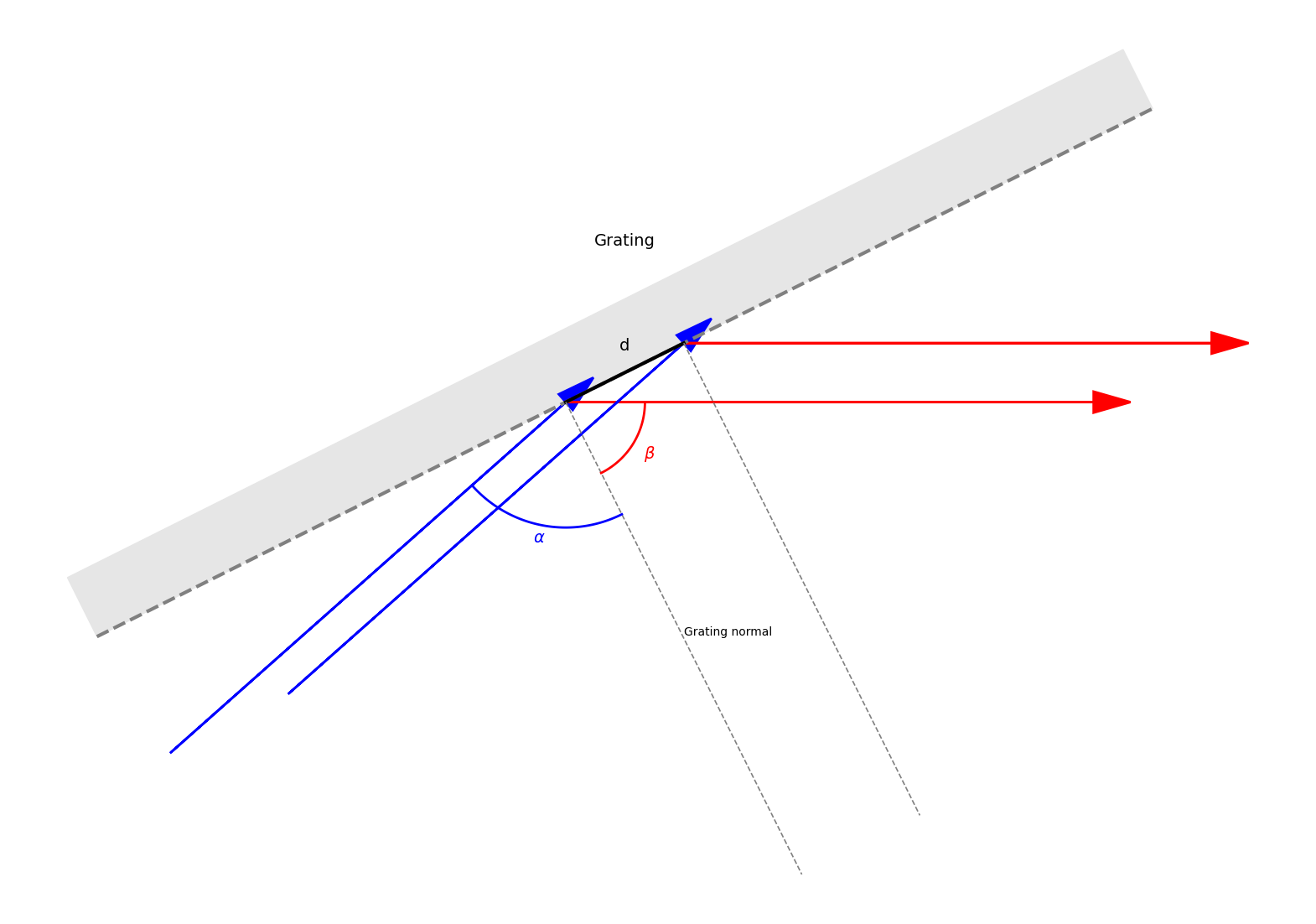
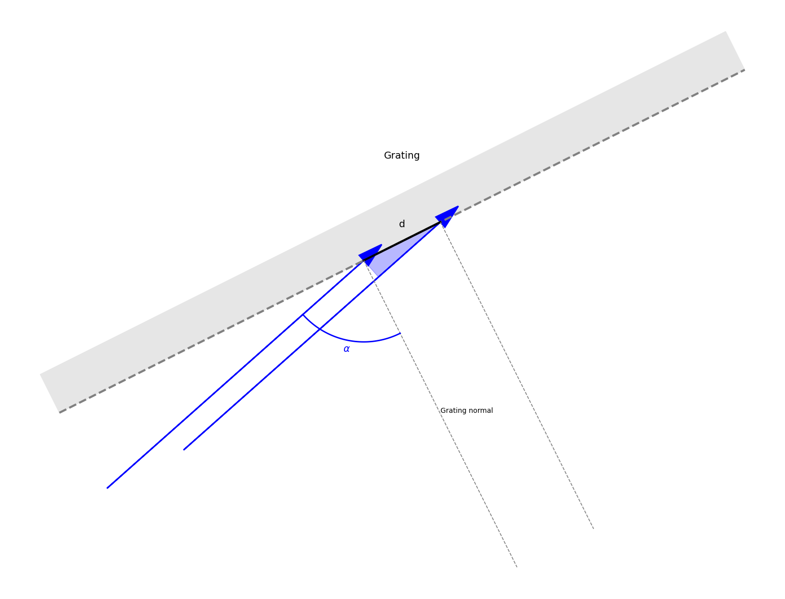
The second incident ray (bottom blue ray) has to travel an extra distance to reach the grating. This extra distance is depicted as the leg of a right triangle with a hypotenuse of length \(d\). Using trigonometry, this extra distance is \(d sin(\alpha)\).

```{python}
#| code-fold: true
# ---------- Plot ----------
fig, ax = plt.subplots(figsize=(20,20))  # bigger figure
ax.set_aspect('equal')
ax.axis('off')
#ax.set_xlim(*xlims)
#ax.set_ylim(*ylims)

## Grating
ax.add_patch(patches.Polygon(grating_poly, closed=True, color=(0.9, 0.9, 0.9, 1)))
ax.plot(x_vals, y_vals, '--', color=(0.5, 0.5, 0.5, 1), lw=3)
ax.text(0.5*(p1[0] + p2[0]),  0.75*(p1[1] + p2[1]),  "Grating",  color=(0, 0, 0, 1), fontsize=14, ha='center', va='center')

## Groove distance
ax.plot([p1[0], p2[0]], [p1[1], p2[1]], ls='solid', color=(0, 0, 0, 1), lw=3)
ax.text(0.5*(p1[0] + p2[0]),  0.55*(p1[1] + p2[1]),  "d",  color=(0, 0, 0, 1), fontsize=14, ha='center', va='center')

## Grating normal
norm_len = 4.0
for p in (p1, p2):
    ax.plot([p[0], p[0] + norm_len * n_hat[0]],
            [p[1], p[1] + norm_len * n_hat[1]],
            ls='--', color='gray', lw=1.2)
#ax.arrow(p1[0], p1[1], 0.9*n_hat[0], 0.9*n_hat[1], head_width=0.09, head_length=0.12, fc='k', ec='k', lw=1.2)
ax.text(p1[0] + 2.0*n_hat[0], p1[1] + 2.0*n_hat[1], 'Grating normal', fontsize=10, ha='left', va='bottom')

## Light rays
for p in (p1, p2):
    start = p - ray_length * inc_dir
    ax.arrow(start[0], start[1], p[0]-start[0], p[1]-start[1], head_width=0.16, head_length=0.28, fc='b', ec=(0, 0, 1, 1), lw=2)
    #ax.arrow(p[0], p[1], ray_length * dif_dir[0], ray_length * dif_dir[1], head_width=0.16, head_length=0.28, fc='r', ec='r', lw=2)

## Label angles
draw_arc_cw(ax, p1, ang_n, ang_inc_in, radius=0.95, color='b', lw=2)  ## α arc
mid_alpha = (ang_n + angle_between(ang_n, ang_inc_in)/2.0)
ax.text(p1[0] + 1.05*np.cos(mid_alpha), p1[1] + 1.05*np.sin(mid_alpha), r"$\alpha$", color='b', fontsize=14, ha='center', va='center')
#draw_arc_short(ax, p1, ang_n, ang_dif, radius=0.6, color='r', lw=2) ## β arc 
#mid_beta  = ang_n + angle_between(ang_n, ang_dif)/2.0
#ax.text(p1[0] + 0.75*np.cos(mid_beta),  p1[1] + 0.75*np.sin(mid_beta),  r"$\beta$",  color='r', fontsize=14, ha='center', va='center')


## Draw triangles
ax.add_patch(patches.Polygon([p1, p2, q_inc], closed=True, color='b', alpha=0.28))


plt.show()
```

Similarly, the second diffracted ray (bottom red ray) has to travel an extra distance of \(d sin(\beta)\).

```{python}
#| code-fold: true
# ---------- Plot ----------
fig, ax = plt.subplots(figsize=(20,20))  # bigger figure
ax.set_aspect('equal')
ax.axis('off')
#ax.set_xlim(*xlims)
#ax.set_ylim(*ylims)

## Grating
ax.add_patch(patches.Polygon(grating_poly, closed=True, color=(0.9, 0.9, 0.9, 1)))
ax.plot(x_vals, y_vals, '--', color=(0.5, 0.5, 0.5, 1), lw=3)
ax.text(0.5*(p1[0] + p2[0]),  0.75*(p1[1] + p2[1]),  "Grating",  color=(0, 0, 0, 1), fontsize=14, ha='center', va='center')

## Groove distance
ax.plot([p1[0], p2[0]], [p1[1], p2[1]], ls='solid', color=(0, 0, 0, 1), lw=3)
ax.text(0.5*(p1[0] + p2[0]),  0.55*(p1[1] + p2[1]),  "d",  color=(0, 0, 0, 1), fontsize=14, ha='center', va='center')

## Grating normal
norm_len = 4.0
for p in (p1, p2):
    ax.plot([p[0], p[0] + norm_len * n_hat[0]],
            [p[1], p[1] + norm_len * n_hat[1]],
            ls='--', color='gray', lw=1.2)
#ax.arrow(p1[0], p1[1], 0.9*n_hat[0], 0.9*n_hat[1], head_width=0.09, head_length=0.12, fc='k', ec='k', lw=1.2)
ax.text(p1[0] + 2.0*n_hat[0], p1[1] + 2.0*n_hat[1], 'Grating normal', fontsize=10, ha='left', va='bottom')

## Light rays
for p in (p1, p2):
    start = p - ray_length * inc_dir
    #ax.arrow(start[0], start[1], p[0]-start[0], p[1]-start[1], head_width=0.16, head_length=0.28, fc='b', ec=(0, 0, 1, 1), lw=2)
    ax.arrow(p[0], p[1], ray_length * dif_dir[0], ray_length * dif_dir[1], head_width=0.16, head_length=0.28, fc='r', ec='r', lw=2)

## Label angles
#draw_arc_cw(ax, p1, ang_n, ang_inc_in, radius=0.95, color='b', lw=2)  ## α arc
#mid_alpha = (ang_n + angle_between(ang_n, ang_inc_in)/2.0)
#ax.text(p1[0] + 1.05*np.cos(mid_alpha), p1[1] + 1.05*np.sin(mid_alpha), r"$\alpha$", color='b', fontsize=14, ha='center', va='center')
draw_arc_short(ax, p1, ang_n, ang_dif, radius=0.6, color='r', lw=2) ## β arc 
mid_beta  = ang_n + angle_between(ang_n, ang_dif)/2.0
ax.text(p1[0] + 0.75*np.cos(mid_beta),  p1[1] + 0.75*np.sin(mid_beta),  r"$\beta$",  color='r', fontsize=14, ha='center', va='center')


## Draw triangles
#ax.add_patch(patches.Polygon([p1, p2, q_inc], closed=True, color='b', alpha=0.28))
ax.add_patch(patches.Polygon([p1, p2, q_dif], closed=True, color='r', alpha=0.28))

plt.show()
```

The total extra distance is \(d sin(\alpha) + d sin(\beta) = d (sin(\alpha) + sin(\beta))\). In order for the diffracted waves to interfere constructively, the total extra distance has to be equal to an integer multiple of the the beam wavelength. Thus,

\[m\lambda = d(\sin\alpha + \sin\beta)\]

Using the grating equation for energy calibration

The grating equation can be used to calculate the theoretical diffracted beam energy by incorporating \(E = hc/\lambda\) and \(k = 1/d\), in which \(k\) is the lines per millimeter in the grating: https://github.com/xraygui/nbs-bl/blob/master/nbs_bl/gGrEqns.py#L55

\[ E = \frac{m k h c}{\sin\alpha + \sin\beta} \]

The \(\alpha\) and \(\beta\) angles are calculated from the PGM and M2 (mirror 2) angles assuming that 0° is defined as the PGM and M2 surfaces being parallel to the beamline floor with the PGM surface facing downwards and the M2 reflective surface facing upwards; if the PGM and M2 are rotated to the same angle, their surfaces are parallel to each other (TODO: check motor position definitions). M2 is lower and more upstream than the PGM.

The real beam energy and associated PGM angle are found by scanning the PGM angle, measuring the associated sample currents from an HOPG reference sample near its 291.65 eV peak, and finding the PGM angle that results in the maximum sample current. Note that because the PGM is being rotated, the beam energy varies with the PGM angle, and the scanned profile should resemble a segment of an HOPG energy scan.

TODO: Find out how the diffraction order is verified. At the moment, the order of magnitude of the sample current is used to qualitatively assess that the first order of diffraction is used, as zero order would produce a significantly brighter signal, and second (or higher) order would produce a signal that is significantly weaker.

By applying offsets to the PGM and M2 angles (floating parameters), the difference between the theoretical energy calculated from the grating equation and the real beam energy at which the maxima were found can be minimized: https://github.com/xraygui/nbs-bl/blob/master/nbs_bl/gGrEqns.py#L100
For a single scan at a particular condition, there can be an infinite number of solutions for the PGM and M2 angle offsets. However, if scans are performed at a variety of conditions, a larger portion of the energy phase space is sampled, and only a single set of offsets can satisfy all conditions. Typically, scans are performed at a variety of constants of fixed foci (CFFs). Alternatively, different standards can be used at different energies, and all of those scans can similarly be used to solve this multidimensional problem.

Constant of fixed focus

The PGM is a focusing grating. RSoXS normally operates at CFF = 1.45, which places the vertical focal point of the beam at the location of RSoXS slits 1. This will maximize energy resolution because the “sub-beams” associated with each energy will be at their narrowest and blend the least with other energies. When scanning HOPG or another material with sharp peaks, the consequence will be that the most intense peak will show maximum intensity relative to other CFFs because it is less convoluted with neighboring lower-intensity peaks.

TODO: Add more details on how CFF works.

Troubleshooting

When troubleshooting issues in the energy calibration, there are some options to consider.

Try using the zero-order beam. In this case, the grating equation is simplified because \(\alpha = \beta\), \(m = 0\), and multiple wavelengths are present in the reflected ray of light. In theory, the true angles of the PGM and M2 have to be equal, so the offsets can be related to each other.

\[\theta_{M2, motor} - \theta_{M2, offset} = \theta_{PGM, motor} - \theta_{PGM, offset}\] \[\theta_{PGM, offset} = \theta_{M2, offset} + (\theta_{PGM, motor} - \theta_{M2, motor})\]

The \(\theta_{M2, motor}\) and \(\theta_{PGM, motor}\) parameters are known and can be treated as a constant. The above equation can be used to verify that the calculated offsets are accurate.