2026-06-12

```{python}
#| code-fold: true
import numpy as np
import matplotlib.pyplot as plt
import matplotlib.cm as cm
import copy

def create_figure(
    number_rows = 1,
    number_columns = 1,
    subplot_size = (3.25, 3.25),
    margin_subplot_size = (0.6, 0.6),
    margin_figure_size = (0.8, 1.2, 0.4, 0.6),
    figure_title = "",
):
    """
    Initializes figure.
    """

    ## Calculate total figure dimensions
    figure_width = (number_columns * subplot_size[0]) + margin_figure_size[0] + margin_figure_size[1] + ((number_columns - 1) * margin_subplot_size[0])
    figure_height = (number_rows * subplot_size[1]) + margin_figure_size[2] + margin_figure_size[3]  + ((number_rows - 1) * margin_subplot_size[1])

    fig, axs = plt.subplots(
        nrows = number_rows, 
        ncols = number_columns, 
        figsize = (figure_width, figure_height), 
        edgecolor = (0, 0, 0, 0), 
        linewidth = 3,
        dpi = 150,
    )
    ## Manually set fixed margins
    fig.subplots_adjust(
        left = margin_figure_size[0] / figure_width, 
        right = 1 - (margin_figure_size[1] / figure_width), 
        top = 1 - (margin_figure_size[2] / figure_height),
        bottom = margin_figure_size[3] / figure_height, 
        wspace = margin_subplot_size[0] / subplot_size[0],
        hspace = margin_subplot_size[1] / subplot_size[1],
    )

    ## Ensure axs always stays a 2D array
    if number_rows == 1 and number_columns == 1: axs = np.array([[axs]])
    if number_rows == 1 and number_columns > 1: axs = axs.reshape(1, number_columns)
    if number_rows > 1 and number_columns == 1: axs = axs.reshape(number_rows, 1)

    fig.suptitle(figure_title, color=(0, 0, 0, 1), fontname="Calibri", size=12)

    return fig, axs


def format_subplot_1d(
    ax,
    plots = [],
    plots_yright = [],
    plots_errorbar = [],
    plots_errorbar_yright = [],
    axvlines = [],
    axhlines = [],
    x_axis_label = None,
    y_axis_label = None,
    yright_axis_label = None,
    xscale = "linear",
    yscale = "linear",
    yrightscale = "linear",
    xlim = {"left": None, "right": None, "auto": False},
    ylim = {"bottom": None, "top": None, "auto": False},
    yrightlim = {"bottom": None, "top": None, "auto": False},
    legend_loc = None,
    border_colors = [(0, 0, 0, 1), (0, 0, 0, 1), (0, 0, 0, 1), (0, 0, 0, 1)]
):
    """
    Formats one 1D subplot.
    """

    yright_conditions = (
        plots_yright
        or plots_errorbar_yright
    )
    if yright_conditions:
        axright = ax.twinx()

    ## Plot data
    plot_settings_default = {
        "marker": "o", 
        "markersize": 0,
        "markerfacecolor": (0, 0, 0, 1), 
        "markeredgecolor": (0, 0, 0, 1), 
        "markeredgewidth": 1,
        "color": (0, 0, 0, 1),
        "linestyle": "solid",
        "linewidth": 2,
    }
    def render_plots(ax, plots, plots_errorbar):
        for plot_type in [plots, plots_errorbar]:
            plot_colors = cm.rainbow(np.linspace(1, 0, len(plot_type)))
            if len(plot_type) == 1: plot_colors = [(0, 0, 0, 1)]
            for index_plot_settings_user, plot_settings_user in enumerate(plot_type):
                plot_settings = {
                    **plot_settings_default, 
                    "markerfacecolor": plot_colors[index_plot_settings_user],
                    "color": plot_colors[index_plot_settings_user],
                    **plot_settings_user
                }
                x = plot_settings.pop("x")
                y = plot_settings.pop("y")
                ax.plot(x, y, **plot_settings)
    render_plots(ax, plots, plots_errorbar)
    if yright_conditions: render_plots(axright, plots_yright, plots_errorbar_yright)
    
    ## Use mostly the same plot default settings for vertical and horizontal lines with a few differences
    line_settings_default = {
        **plot_settings_default,
        "color": (0.5, 0.5, 0.5, 1),
        "linestyle": "dotted",
    }
    for line_type in [axvlines, axhlines]:
        plot_colors = cm.rainbow(np.linspace(1, 0, len(line_type)))
        if len(line_type) == 1: plot_colors = [(0.5, 0.5, 0.5, 1)]
        for index_line_settings_user, line_settings_user in enumerate(line_type):
            line_settings = {
                **line_settings_default, 
                "markerfacecolor": plot_colors[index_line_settings_user],
                "color": plot_colors[index_line_settings_user],
                **line_settings_user
            }
            if line_type is axvlines: ax.axvline(**line_settings)
            else: ax.axhline(**line_settings)

    ## Label axes
    if x_axis_label:
        x_axis_label_copy = copy.deepcopy(x_axis_label)
        xlabel = x_axis_label_copy.pop("xlabel")
        ax.set_xlabel(xlabel, **x_axis_label_copy)
    if y_axis_label:
        y_axis_label_copy = copy.deepcopy(y_axis_label)
        ylabel = y_axis_label_copy.pop("ylabel")
        ax.set_ylabel(ylabel, **y_axis_label_copy)
    if yright_axis_label:
        yright_axis_label_copy = copy.deepcopy(yright_axis_label)
        yrightlabel = yright_axis_label_copy.pop("ylabel")
        axright.set_ylabel(yrightlabel, **yright_axis_label_copy)

    ## Axes scaling and ranges
    ax.set_xscale(xscale)
    ax.set_yscale(yscale)
    if yright_conditions: axright.set_yscale(yrightscale)
    ax.set_xlim(**xlim)
    ax.set_ylim(**ylim)
    if yright_conditions: axright.set_ylim(**yrightlim)

    ## Border formatting
    def border_formatting(ax, axes_tick_parms = [3, 0]):
        for index_border, border in enumerate(["left", "right", "top", "bottom"]):
            ax.spines[border].set_linewidth(2)
            ax.spines[border].set_color(border_colors[index_border])
        for index_axis, axis in enumerate(["x", "y"]): ax.tick_params(axis=axis, colors=border_colors[axes_tick_parms[index_axis]], width=2)
        ax.tick_params(axis='both', which='major', labelsize=10)
    border_formatting(ax)
    if yright_conditions: border_formatting(axright, axes_tick_parms = [3, 1])

    ## Legends - display labels from plots with optional positioning
    handles, labels = ax.get_legend_handles_labels()
    if yright_conditions:
        handles_r, labels_r = axright.get_legend_handles_labels()
        handles.extend(handles_r)
        labels.extend(labels_r)
    
    if handles and labels and legend_loc:
        ax.legend(handles, labels, loc=legend_loc, fontsize=9, frameon=True, 
                 fancybox=False, edgecolor=(0, 0, 0, 1), framealpha=0.95)
```

Axis SXR-40 camera commissioning

Background

An in-vacuum sCMOS camera was purchased from Axis Photonique to be used in the upcoming RSoXS chamber upgrade. The in-vacuum form-factor will translate over a wide linear and angular range to perform standard SAXS/WAXS measurements along with reflectivity and CDSAXS. The sCMOS EUV-enhanced sensor will have faster a faster frame rate and higher quantum efficiency than the current Greateyes CCD camera, enabling higher measurement throughput and lower X-ray dose on the sample.

Bench testing setup

The detectors were received on July 11, 2026.

For in-air bench testing, it is important to minimize contamination on the camera, as the entire body will be placed inside the ultra-high-vacuum (UHV) beamline. Gloves were worn at all times while handling the camera, and they were changed frequently. The testing bench was decluttered and wiped clean with ethanol. A large piece of UHV foil was placed on the working surface. For initial electronics connection testing, only the back side of the plastic wrapping on the camera was cut to expose the electronics ports, while leaving the remainder of the camera shrouded inside the plastic wrapping. While testing image capture, the plastic wrapping was cut from the top such that the camera sits on top of the plastic wrapping which is on top of the UHV foil that lines the test bench. The cooling lines and mini flanges were covered with UHV foil to protect the knife edge of the foil and prevent dust and debris from going inside the cooling lines. When the detector was not actively in use, a box with UHV foil lined on the inside was placed over the detector with a “DO NOT TOUCH” not on top.

The detector’s optical ports were covered by metal caps, and most cable ends were covered with plastic caps. These caps were saved in a plastic vial.

For short-term bench tests, an HP Z6 tower with Windows operating system was used to install the frame grabber card. The setup of a longer-term Windows machine dedicated for bench tests is documented in a Jira ticket (https://jira.nsls2.bnl.gov/browse/SPEC-157). Although the electronics are capable of working in USB, only the CameraLink mode was available because of how the electronics were concealed in the airbox. The USB mode would have been available for an equivalent flange-mounted detector.

Only the out-of-vacuum cables were connected directly to the detector. The duplex optical cable was connected directly to the detector. The other ends of the duplex optical cables were connected into the optical-to-CameraLink converter box, and this box was connected to the frame grabber card that was installed into the Windows desktop tower machine. The red-colored cables and ports are for the BASE signal, which supports communication and part of the image feed. The other path is for the FULL signal, which supports the image feed.

The thermoelectric cooler (TEC) should never be started unless the camera is under vacuum. Ideally, it is still preferable to run water through the cooling lines during bench tests to keep the sensor stable at room temperature. However, to minimize the bench test setup profile and also avoid getting the cooling lines wet prior to UHV installation, no coolant was flown through the cooling lines. The camera was only powered on for up to 15 min at any time followed by at least 2 h of being powered off so that the sensor temperature changes minimally while the camera is on and fully cools down before the next power-on. The camera body enclosure was touched gently to monitor the temperature that way, and the temperature readouts from the software application were saved along with images.

Frame rate vs. ROI

The physical setup was the same as that used for dark images; see subsection below. For all sets of images, the exposure time was set to 10 us in the “Camera” tab; this is the fastest exposure time possible on the detector. Also in the “Camera” tab, the region of interest (ROI) size was set by selecting “Manual” –> “Single”, unchecking “Fast ROI”, adjusting the “Width” and “Height” of the ROI, and clicking “Set ROI”. Both the “StartX” and “StartY” of the ROI always were set to 0. Under the “Acquisition” tab, “Use Fixed Path” was selected, the “Path” was set to load images into the desired folder in File Explorer, “Total Frame” was set to 300, “Image Capture” –> “Format” was set to TIF, and “Save To” was selected to “To RAM” with “Frames per Stack” as 1 and “RAM Buffer” as “Manual”. The “To RAM” setting helped insure that the frame rate is not artificially slowed down by the time taken to write images to disk. Images were captured by clicking “Capture” under “Image Capture”.

300 images were captured at each ROI to determine the average frame rate per ROI.

The true timestamps of the images were not easily available via the front-end GUI software. Thus, they were estimated using the file and folder names. The folder name for each replicate set contained the timestamp at the beginning of the image capture. The file names for each individual image contained timestamps from after all images were captured and reflected when those images were transferred from RAM to disk. To estimate the timestamp of each image, the timestamp in the folder name was approximated to be the timestamp of the first image, the timestamp in the first image file name was estimated to be the timestamp of the (n+1)th image, and all other image timestamps were interpolated between the start and (n+1)th timestamp. It was assumed that the file names of the images reflected the chronological order in which the images were captured, and timestamp interpolation preserved that relative order of images.

It is important to note that this method of timestamp estimation assumes that the image capture times were spaced perfectly evenly, and that no frames were dropped. A large number of replicate images (300) helps ensure that the estimated frame rate is close to the true frame rate, assuming that a very small portion of frames or zero frames were dropped during acquisition. After setting up EPICS and Bluesky control of this detector and extracting true timestamps, it will be helpful to create a histogram of timestamps to verify that minimal-to-no frames are dropped, and that the variance of interval times is close-to-zero, as was assumed for bench tests.

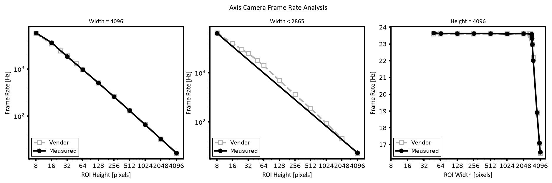
The average frame rate was calculated as 1 divided by the average inter-frame interval time. The plots below show that all estimated frame rates from bench testing at NSLS II agree with the frame rates calculated by Axis during the factory acceptance tests.

```{python}
#| code-fold: true
import numpy as np
import matplotlib.pyplot as plt
from matplotlib import cm

vendor_h_full_x = np.array([8, 16, 24, 32, 48, 64, 128, 256, 512, 1024, 2048, 4096], dtype=float)
vendor_h_full_y = np.array([5700.0, 3450.0, 2450.0, 1900.0, 1300.0, 1000.0, 510.0, 260.0, 130.0, 66.0, 33.0, 16.5], dtype=float)
vendor_h_reduced_x = np.array([8, 16, 24, 32, 48, 64, 128, 256, 512, 1024, 2048, 4096], dtype=float)
vendor_h_reduced_y = np.array([6500.0, 4000.0, 3000.0, 2500.0, 1800.0, 1400.0, 700.0, 360.0, 190.0, 95.0, 46.0, 23.4], dtype=float)
vendor_w_scan_x = np.array([48, 64, 128, 256, 512, 1024, 2048, 2560, 2688, 2752, 2816, 2864, 2880, 2944, 3072, 3584, 3968, 4096], dtype=float)
vendor_w_scan_y = np.array([23.6, 23.6, 23.6, 23.6, 23.6, 23.6, 23.6, 23.6, 23.6, 23.5, 23.5, 23.4, 23.3, 23.0, 22.2, 18.9, 17.1, 16.5], dtype=float)

measured_h_full_x = np.array([8, 16, 32, 64, 128, 256, 512, 1024, 2048, 4096], dtype=float)
measured_h_full_y = np.array([5882.352941, 3663.003663, 1851.851852, 974.658869, 510.204082, 260.416667, 131.354262, 65.980470, 33.018556, 16.553551], dtype=float)
measured_h_reduced_x = np.array([8, 4096, 4096, 4096, 4096, 4096, 4096, 4096, 4096], dtype=float)
measured_h_reduced_y = np.array([6410.256410, 23.661359, 23.614981, 23.622233, 23.618328, 23.623907, 23.598263, 23.627815, 23.584906], dtype=float)
measured_w_scan_x = np.array([48, 64, 128, 256, 512, 1024, 2048, 2864, 2880, 2896, 2944, 3072, 3584, 3968, 4096], dtype=float)
measured_w_scan_y = np.array([23.661359, 23.614981, 23.622233, 23.618328, 23.623907, 23.598263, 23.627815, 23.584906, 23.487411, 23.319264, 22.969497, 22.015279, 18.913245, 17.085255, 16.553551], dtype=float)

fig, axs = create_figure(
    number_rows=1,
    number_columns=3,
    subplot_size=(3.5, 3.0),
    margin_subplot_size=(0.6, 0.6),
    margin_figure_size=(0.8, 0.4, 0.6, 0.8),
    figure_title="Axis Camera Frame Rate Analysis"
)

power_of_2_ticks = [2**i for i in range(3, 13)]
power_of_2_labels = [str(t) for t in power_of_2_ticks]

ax = axs[0, 0]
plots_list_h_full = [
    {"x": vendor_h_full_x, "y": vendor_h_full_y, "linestyle": "--", "linewidth": 2.5, "color": (0.7, 0.7, 0.7, 1), "marker": "s", "markersize": 7, "markerfacecolor": (1, 1, 1, 1), "markeredgecolor": (0.7, 0.7, 0.7, 1), "markeredgewidth": 1.5, "label": "Vendor"},
    {"x": measured_h_full_x, "y": measured_h_full_y, "linestyle": "-", "linewidth": 2.5, "color": (0, 0, 0, 1), "marker": "o", "markersize": 6, "markerfacecolor": (0, 0, 0, 1), "markeredgecolor": (0, 0, 0, 1), "markeredgewidth": 1.5, "label": "Measured"},
]
format_subplot_1d(ax, plots=plots_list_h_full, x_axis_label={"xlabel": "ROI Height [pixels]", "fontsize": 11, "fontname": "Calibri"}, y_axis_label={"ylabel": "Frame Rate [Hz]", "fontsize": 11, "fontname": "Calibri"}, xscale="log", yscale="log", legend_loc="lower left")
ax.set_xticks(power_of_2_ticks)
ax.set_xticklabels(power_of_2_labels)
ax.set_title("Width = 4096", fontsize=10, fontname="Calibri")

ax = axs[0, 1]
plots_list_h_reduced = [
    {"x": vendor_h_reduced_x, "y": vendor_h_reduced_y, "linestyle": "--", "linewidth": 2.5, "color": (0.7, 0.7, 0.7, 1), "marker": "s", "markersize": 7, "markerfacecolor": (1, 1, 1, 1), "markeredgecolor": (0.7, 0.7, 0.7, 1), "markeredgewidth": 1.5, "label": "Vendor"},
    {"x": measured_h_reduced_x, "y": measured_h_reduced_y, "linestyle": "-", "linewidth": 2.5, "color": (0, 0, 0, 1), "marker": "o", "markersize": 6, "markerfacecolor": (0, 0, 0, 1), "markeredgecolor": (0, 0, 0, 1), "markeredgewidth": 1.5, "label": "Measured"},
]
format_subplot_1d(ax, plots=plots_list_h_reduced, x_axis_label={"xlabel": "ROI Height [pixels]", "fontsize": 11, "fontname": "Calibri"}, y_axis_label={"ylabel": "Frame Rate [Hz]", "fontsize": 11, "fontname": "Calibri"}, xscale="log", yscale="log", legend_loc="lower left")
ax.set_xticks(power_of_2_ticks)
ax.set_xticklabels(power_of_2_labels)
ax.set_title("Width < 2865", fontsize=10, fontname="Calibri")

ax = axs[0, 2]
plots_list_w = [
    {"x": vendor_w_scan_x, "y": vendor_w_scan_y, "linestyle": "--", "linewidth": 2.5, "color": (0.7, 0.7, 0.7, 1), "marker": "s", "markersize": 7, "markerfacecolor": (1, 1, 1, 1), "markeredgecolor": (0.7, 0.7, 0.7, 1), "markeredgewidth": 1.5, "label": "Vendor"},
    {"x": measured_w_scan_x, "y": measured_w_scan_y, "linestyle": "-", "linewidth": 2.5, "color": (0, 0, 0, 1), "marker": "o", "markersize": 6, "markerfacecolor": (0, 0, 0, 1), "markeredgecolor": (0, 0, 0, 1), "markeredgewidth": 1.5, "label": "Measured"},
]
format_subplot_1d(ax, plots=plots_list_w, x_axis_label={"xlabel": "ROI Width [pixels]", "fontsize": 11, "fontname": "Calibri"}, y_axis_label={"ylabel": "Frame Rate [Hz]", "fontsize": 11, "fontname": "Calibri"}, xscale="log", yscale="linear", legend_loc="lower left")
ax.set_xticks(power_of_2_ticks)
ax.set_xticklabels(power_of_2_labels)
ax.set_title("Height = 4096", fontsize=10, fontname="Calibri")

plt.show()
```

Dark current rate and readout noise

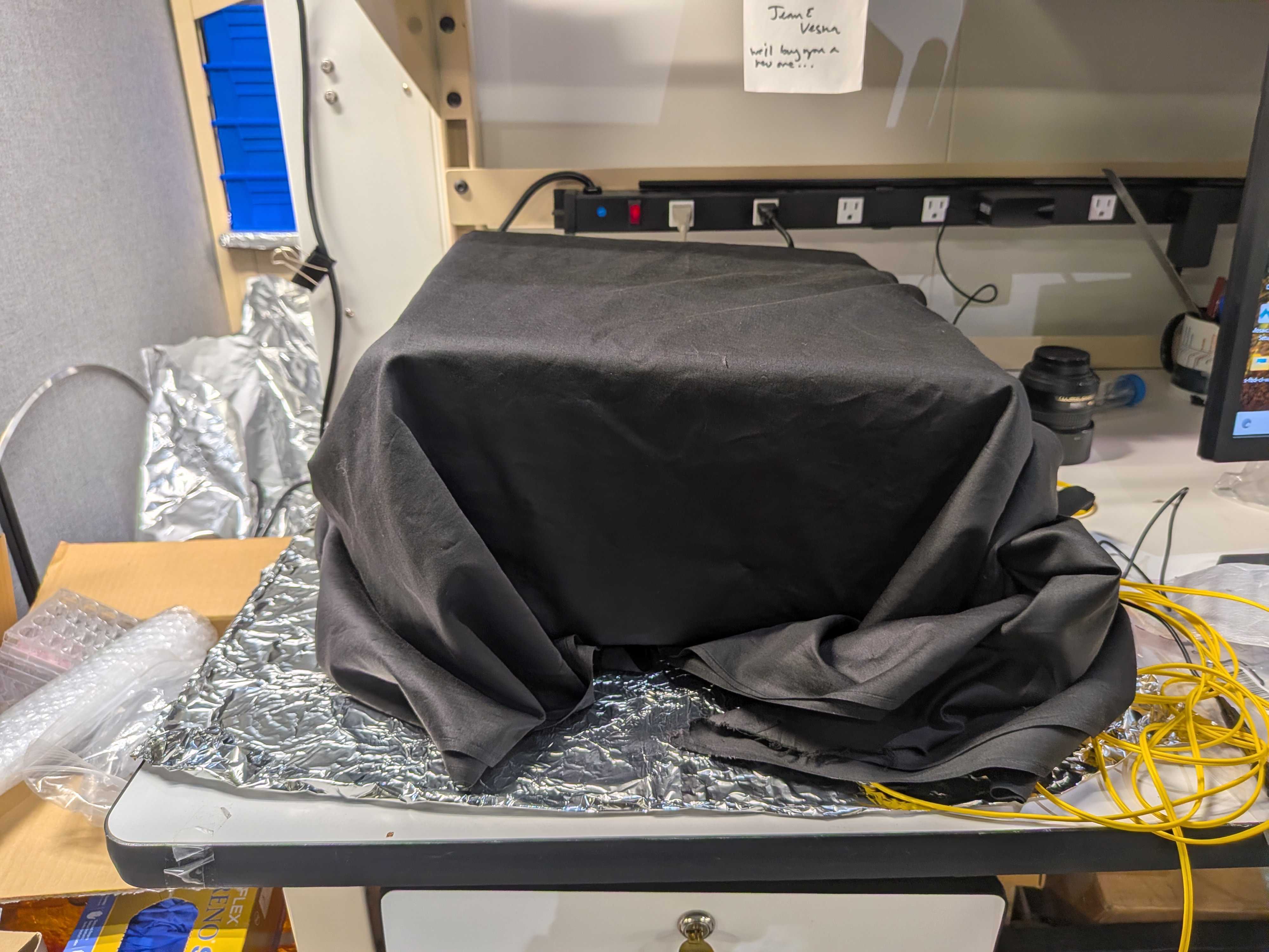
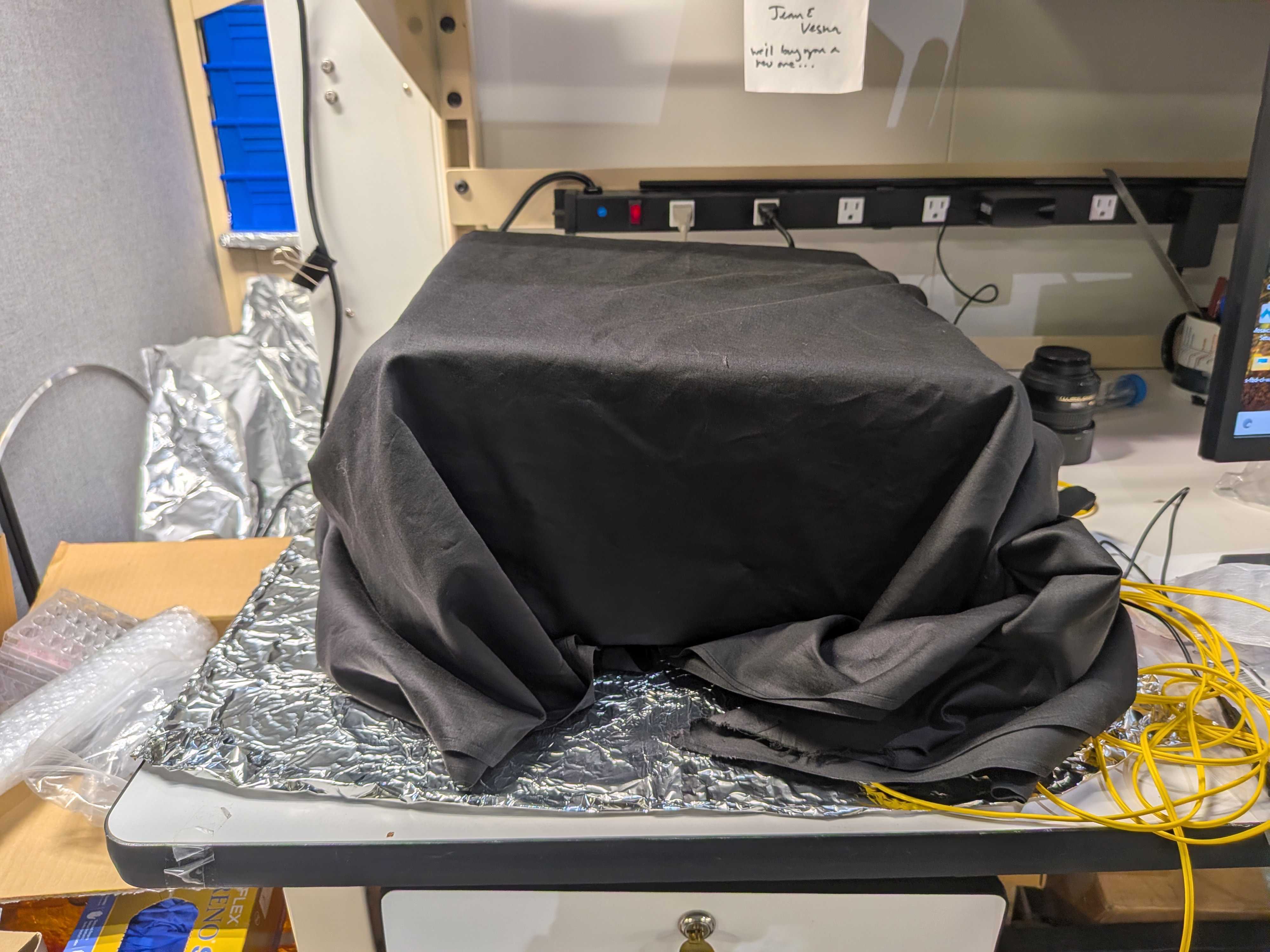
All dark images were captured with the protective window and lens adaptor cap shut. Additionally, the same box used to protect the detector from dust and debris was lightly placed over the camera, and a blackout fabric was shrouded the box and tucked into the open spaces near the bottom of the box and cables. However, it is important to not tuck the fabric too far in, as the dust from the fabric can contaminate the detector body. At a 1 s exposure time at low gain, the average counts with the box + fabric were ~100, whereas the counts were ~108 without the box + fabric.

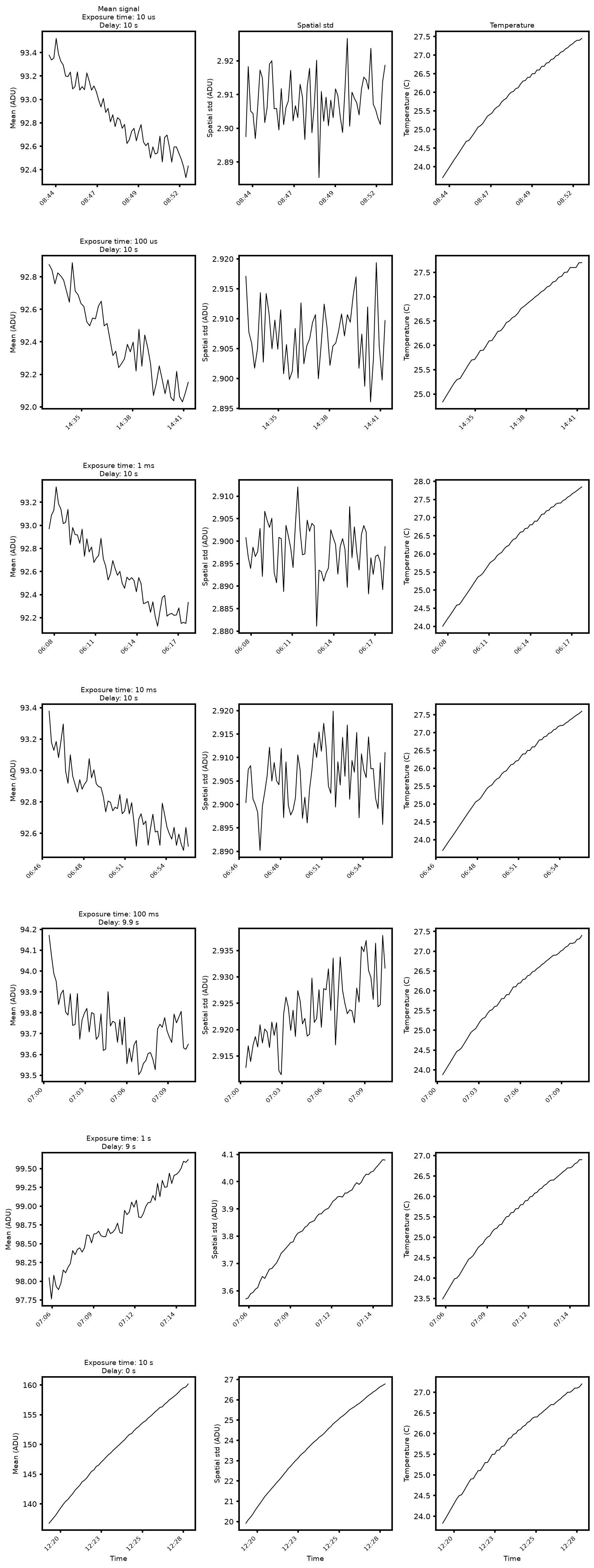
The sensor was not actively cooled during bench tests, so it was important to account for temperature drift while the camera was turned on. The sensor temperature naturally increased with time even when the camera was sitting idly powered on, and the temperature can increase further while reading out images.

In an attempt to capture all sets of images under identical conditions, each exposure time stack was captured immediately after the camera was powered on. For each replicate image, the exposure time + delay time was set to a constant of 10 s. 60 replicate images were captured at exposure times ranging from 10 us to 10 s and the appropriate corresponding delay times. This was done in the “Acquisition” tab by setting Total Frame: 60 and e.g., Time-Lapse Photogrpahy Interval time: 0 m 9 s 0 ms for a 1 s exposure time. The camera was then powered off for at least 2 h and left uncovered so that the natural air flow would allow the instrument to cool down.

Image timestaps were estimated as described in the frame rate calculation subsection. Sensor temperatures also were exported along with the data, and the temperatures shown below were interpolated for each image timestamp.

```{python}
#| code-fold: true
# ── Imports ────────────────────────────────────────────────────────────────
from pathlib import Path
from collections import Counter
import re, copy, yaml

import numpy as np
import pandas as pd
import matplotlib.pyplot as plt
import matplotlib.cm as cm
import matplotlib.dates as mdates
import xray_loaders
import dask

# ── Run roots (sorted by exposure time, shortest → longest) ───────────────
_BASE = Path(r"G:\Shared drives\NISTPostdoc\CharacterizationData\BeamTime\2026-06-12_axis_bench_testing")

def _parse_exp_s(path):
    m = re.search(r"exp(\d+)(us|ms|s)", path.name.lower())
    if not m:
        return np.inf
    v, u = float(m.group(1)), m.group(2)
    return v * {"us": 1e-6, "ms": 1e-3, "s": 1.0}[u]

run_roots = sorted([
    _BASE / "2026-06-26" / "dark_lowgain_exp1ms_delay9s999ms",
    _BASE / "2026-06-27" / "dark_lowgain_exp10ms_delay9s990ms",
    _BASE / "2026-07-05" / "dark_lowgain_exp1s_delay9s",
    _BASE / "2026-07-02" / "dark_lowgain_exp10s_delay0s",
    _BASE / "2026-07-02" / "dark_lowgain_exp10us_delay10s",
    _BASE / "2026-07-02" / "dark_lowgain_exp100us_delay10s",
    _BASE / "2026-07-03" / "dark_lowgain_exp100ms_delay9s900ms",
], key=_parse_exp_s)

# ── Helpers ────────────────────────────────────────────────────────────────
def _locate_files(run_root):
    tifs = sorted(run_root.rglob("*.tif"))
    if not tifs:
        raise FileNotFoundError(f"No TIFFs under {run_root}")
    image_dir = Counter(t.parent for t in tifs).most_common(1)[0][0]
    csvs = sorted(run_root.rglob("*temperature*.csv"))
    if not csvs:
        raise FileNotFoundError(f"No temperature CSV under {run_root}")
    yamls = sorted(run_root.rglob("*axis_mosaic_metadata*.yaml"))
    if not yamls:
        yaml_path = run_root / "axis_mosaic_metadata.yaml"
        with open(yaml_path, "w") as f:
            yaml.dump({
                "axis_mosaic_exposure_time": f"{_parse_exp_s(run_root):.6g} seconds",
                "axis_mosaic_scan_type":     "dark",
                "axis_mosaic_interval_time": "0 seconds",
                "axis_mosaic_binning":       "1x1",
            }, f)
        yamls = [yaml_path]
    return image_dir, csvs[0], yamls[0]

def _robust_z(arr):
    med = np.median(arr)
    mad = np.median(np.abs(arr - med))
    return 0.6745 * (arr - med) / mad if mad > 0 else np.zeros_like(arr, dtype=float)

def _analyze_run(run_root):
    image_dir, csv_path, yaml_path = _locate_files(run_root)
    ds = xray_loaders.load_axis_mosaic_scan(
        image_dir            = image_dir,
        temperature_csv_path = csv_path,
        metadata_yaml_path   = yaml_path,
    )
    mean_arr, std_arr = dask.compute(
        ds["image"].mean(dim=["pix_y", "pix_x"]),
        ds["image"].std(dim=["pix_y", "pix_x"]),
    )
    mean_arr = mean_arr.values.astype(float)
    std_arr  = std_arr.values.astype(float)
    temp_arr = ds["sensor_temperature"].values.astype(float)
    time_arr = pd.to_datetime(ds["time"].values)
    flagged  = (np.abs(_robust_z(mean_arr)) > 5.0) | (np.abs(_robust_z(std_arr)) > 6.0)
    return pd.DataFrame({
        "time":          time_arr,
        "temperature_C": temp_arr,
        "mean_adu":      mean_arr,
        "std_adu":       std_arr,
        "flagged":       flagged,
    })

def _format_run_label(run_name):
    """Parse 'exp10us_delay10s' -> 'Exposure time: 10 us\nDelay: 10 s'."""
    short = re.sub(r"^dark_lowgain_", "", run_name)
    unit_map = {"us": "us", "ms": "ms", "s": "s"}

    m_exp = re.search(r"exp(\d+)(us|ms|s)", short)
    exp_str = f"{int(m_exp.group(1))} {unit_map[m_exp.group(2)]}" if m_exp else "?"

    m_delay = re.search(r"delay(\d+)s(?:(\d+)ms)?", short)
    if m_delay:
        total_s = int(m_delay.group(1)) + (int(m_delay.group(2)) / 1000.0 if m_delay.group(2) else 0)
        rounded = round(total_s)
        delay_str = f"{rounded} s" if abs(total_s - rounded) < 0.05 else f"{total_s:.1f} s"
    else:
        delay_str = "?"

    return f"Exposure time: {exp_str}\nDelay: {delay_str}"

# ── Load data ─────────────────────────────────────────────────────────────
tables     = {rr.name: _analyze_run(rr) for rr in run_roots}
run_labels = [rr.name for rr in run_roots]

# ── Build figure ──────────────────────────────────────────────────────────
n_runs = len(run_roots)

fig, axs = create_figure(
    number_rows         = n_runs,
    number_columns      = 3,
    subplot_size        = (2.8, 2.8),
    margin_subplot_size = (0.8, 1.3),
    margin_figure_size  = (1.4, 0.6, 0.8, 1.0),
)

_black = (0, 0, 0, 1)
_red   = (0.8, 0.1, 0.1, 0.9)

col_ykeys   = ["mean_adu",    "std_adu",           "temperature_C"   ]
col_ylabels = ["Mean (ADU)", "Spatial std (ADU)", "Temperature (C)"]
col_headers = ["Mean signal", "Spatial std",       "Temperature"     ]

for row, run_name in enumerate(run_labels):
    dfr     = tables[run_name]
    flagged = dfr["flagged"].to_numpy()
    last    = (row == n_runs - 1)
    label   = _format_run_label(run_name)

    for col, (ykey, ylabel_text, col_hdr) in enumerate(zip(col_ykeys, col_ylabels, col_headers)):
        ax = axs[row, col]

        format_subplot_1d(
            ax,
            plots = [{
                "x":         dfr["time"],
                "y":         dfr[ykey],
                "linewidth": 1,
                "color":     _black,
            }],
            x_axis_label = {"xlabel": "Time", "fontsize": 9} if last else None,
            y_axis_label = {"ylabel": ylabel_text, "fontsize": 9},
        )

        if flagged.any():
            ax.scatter(
                dfr.loc[flagged, "time"],
                dfr.loc[flagged, ykey],
                color = _red, s = 18, marker = "x", zorder = 5, linewidths = 1.5,
            )

        if row == 0 and col == 0:
            ax.set_title(f"{col_hdr}\n{label}", fontsize = 9, color = _black, pad = 5)
        elif row == 0:
            ax.set_title(col_hdr, fontsize = 9, color = _black, pad = 5)
        elif col == 0:
            ax.set_title(label, fontsize = 9, color = _black, pad = 5)

        ax.xaxis.set_major_formatter(mdates.DateFormatter("%H:%M"))
        plt.setp(ax.get_xticklabels(), rotation = 45, ha = "right", fontsize = 8)

plt.show()
```

Optional query helpers are unavailable. Install bluesky_tiled_plugins or databroker for advanced search support.

G:\Shared drives\NISTPostdoc\DeliverablesReferences\Codebases\xray_loaders\src\xray_loaders\axis_mosaic_loader.py:441: UserWarning: Axis Mosaic frame timestamps are interpolated, not hardware-measured. Folder '20260702-084341448' → t_start=2026-07-02 08:43:41.448000; earliest file 'TUC-20260702085333454.tif' → t_end_anchor=2026-07-02 08:53:33.454000; estimated interval=9.866767 s across 60 frames. See parse_axis_mosaic_image_timestamps docstring for full assumptions.
  image_paths, image_timestamps = parse_axis_mosaic_image_timestamps(image_dir)
G:\Shared drives\NISTPostdoc\DeliverablesReferences\Codebases\xray_loaders\src\xray_loaders\axis_mosaic_loader.py:441: UserWarning: Axis Mosaic frame timestamps are interpolated, not hardware-measured. Folder '20260702-143340836' → t_start=2026-07-02 14:33:40.836000; earliest file 'TUC-20260702144142480.tif' → t_end_anchor=2026-07-02 14:41:42.480000; estimated interval=9.829469 s across 49 frames. See parse_axis_mosaic_image_timestamps docstring for full assumptions.
  image_paths, image_timestamps = parse_axis_mosaic_image_timestamps(image_dir)
G:\Shared drives\NISTPostdoc\DeliverablesReferences\Codebases\xray_loaders\src\xray_loaders\axis_mosaic_loader.py:441: UserWarning: Axis Mosaic frame timestamps are interpolated, not hardware-measured. Folder '20260626-060816491' → t_start=2026-06-26 06:08:16.491000; earliest file 'TUC-20260626061808512.tif' → t_end_anchor=2026-06-26 06:18:08.512000; estimated interval=9.867017 s across 60 frames. See parse_axis_mosaic_image_timestamps docstring for full assumptions.
  image_paths, image_timestamps = parse_axis_mosaic_image_timestamps(image_dir)
G:\Shared drives\NISTPostdoc\DeliverablesReferences\Codebases\xray_loaders\src\xray_loaders\axis_mosaic_loader.py:441: UserWarning: Axis Mosaic frame timestamps are interpolated, not hardware-measured. Folder '20260627-064632852' → t_start=2026-06-27 06:46:32.852000; earliest file 'TUC-20260627065624823.tif' → t_end_anchor=2026-06-27 06:56:24.823000; estimated interval=9.866183 s across 60 frames. See parse_axis_mosaic_image_timestamps docstring for full assumptions.
  image_paths, image_timestamps = parse_axis_mosaic_image_timestamps(image_dir)
G:\Shared drives\NISTPostdoc\DeliverablesReferences\Codebases\xray_loaders\src\xray_loaders\axis_mosaic_loader.py:441: UserWarning: Axis Mosaic frame timestamps are interpolated, not hardware-measured. Folder '20260703-070050568' → t_start=2026-07-03 07:00:50.568000; earliest file 'TUC-20260703071041069.tif' → t_end_anchor=2026-07-03 07:10:41.069000; estimated interval=9.841683 s across 60 frames. See parse_axis_mosaic_image_timestamps docstring for full assumptions.
  image_paths, image_timestamps = parse_axis_mosaic_image_timestamps(image_dir)
G:\Shared drives\NISTPostdoc\DeliverablesReferences\Codebases\xray_loaders\src\xray_loaders\axis_mosaic_loader.py:441: UserWarning: Axis Mosaic frame timestamps are interpolated, not hardware-measured. Folder '20260705-070601599' → t_start=2026-07-05 07:06:01.599000; earliest file 'TUC-20260705071552277.tif' → t_end_anchor=2026-07-05 07:15:52.277000; estimated interval=9.844633 s across 60 frames. See parse_axis_mosaic_image_timestamps docstring for full assumptions.
  image_paths, image_timestamps = parse_axis_mosaic_image_timestamps(image_dir)
G:\Shared drives\NISTPostdoc\DeliverablesReferences\Codebases\xray_loaders\src\xray_loaders\axis_mosaic_loader.py:441: UserWarning: Axis Mosaic frame timestamps are interpolated, not hardware-measured. Folder '20260702-121921565' → t_start=2026-07-02 12:19:21.565000; earliest file 'TUC-20260702122918762.tif' → t_end_anchor=2026-07-02 12:29:18.762000; estimated interval=9.953283 s across 60 frames. See parse_axis_mosaic_image_timestamps docstring for full assumptions.
  image_paths, image_timestamps = parse_axis_mosaic_image_timestamps(image_dir)

Gain

A 50 mm Nikon F-mount Nikon lens (https://www.gsaadvantage.gov/advantage/ws/catalog/product_detail?gsin=11000006516465) was attached to the camera for light-containing images. Although the lens is not necessary, it produced images to visually inspect the quality of the performance.

Software setup: EPICS and Bluesky

Jira ticket: https://jira.nsls2.bnl.gov/browse/SPEC-154

A dedicated Linux machine is being set up for the detector.

Image performance characterization

Vacuum testing

In light of the recent and older vacuum issues encountered for the Greateyes CCD camera, the new Axis SXR-40 camera will be characterized by the Vacuum Group upon arrival.

Mounting into current RSoXS station

Due to the recent issues with the Greateyes CCD camera (e.g., cooling line leak, contaminated sensor), there are plans to install the new Axis SXR-40 into the current RSoXS chamber for the meantime before the new RSoXS chamber is installed.

With the help of a BNL engineer, a new mount was designed that can be attached to the existing translation assembly for the Greateyes cameras. This allows the same motors to be reused and for the new camera to fit into the geometry of the current RSoXS chamber.

The mount was designed such that in the retracted state, the camera has similar clearance from the beam as the existing Greateyes detector which is sufficient for dithered and undithered beam sizes.